Classification
In this notebook we demonstrate how to perform inference for Gaussian process models with non-Gaussian likelihoods via maximum a posteriori (MAP). We focus on a classification task here.
from flax import nnx
import jax

# Enable Float64 for more stable matrix inversions.
from jax import config
import jax.numpy as jnp
import jax.random as jr
import jax.scipy as jsp
from jaxtyping import (
    Array,
    Float,
    install_import_hook,
)
import matplotlib.pyplot as plt
import numpyro.distributions as npd
import optax as ox

from examples.utils import use_mpl_style
from gpjax.linalg import (
    PSD,
    lower_cholesky,
    solve,
)

config.update("jax_enable_x64", True)


with install_import_hook("gpjax", "beartype.beartype"):
    import gpjax as gpx
    from gpjax.parameters import Parameter


identity_matrix = jnp.eye

# set the default style for plotting
use_mpl_style()

key = jr.key(42)
cols = plt.rcParams["axes.prop_cycle"].by_key()["color"]
Dataset
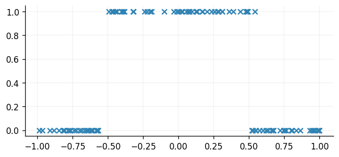
With the necessary modules imported, we simulate a dataset with inputs sampled uniformly on and corresponding binary outputs
We store our data as a GPJax Dataset and create test inputs for
later.
key, subkey = jr.split(key)
x = jr.uniform(key, shape=(100, 1), minval=-1.0, maxval=1.0)
y = 0.5 * jnp.sign(jnp.cos(3 * x + jr.normal(subkey, shape=x.shape) * 0.05)) + 0.5

D = gpx.Dataset(X=x, y=y)

xtest = jnp.linspace(-1.0, 1.0, 500).reshape(-1, 1)

fig, ax = plt.subplots()
ax.scatter(x, y)
<matplotlib.collections.PathCollection at 0x7efdeaa0d190>
MAP inference
We begin by defining a Gaussian process prior with a radial basis function (RBF) kernel, chosen for the purpose of exposition. Since our observations are binary, we choose a Bernoulli likelihood with a probit link function.
kernel = gpx.kernels.RBF()
meanf = gpx.mean_functions.Constant()
prior = gpx.gps.Prior(mean_function=meanf, kernel=kernel)
likelihood = gpx.likelihoods.Bernoulli(num_datapoints=D.n)
We construct the posterior through the product of our prior and likelihood.
<class 'gpjax.gps.NonConjugatePosterior'>
Whilst the latent function is Gaussian, the posterior distribution is non-Gaussian since our generative model first samples the latent GP and propagates these samples through the likelihood function's inverse link function. This step prevents us from being able to analytically integrate the latent function's values out of our posterior, and we must instead adopt alternative inference techniques. We begin with maximum a posteriori (MAP) estimation, a fast inference procedure to obtain point estimates for the latent function and the kernel's hyperparameters by maximising the marginal log-likelihood.
We can obtain a MAP estimate by optimising the log-posterior density with Optax's optimisers.
optimiser = ox.adam(learning_rate=0.01)
opt_posterior, history = gpx.fit(
    model=posterior,
    # we use the negative lpd as we are minimising
    objective=lambda p, d: -gpx.objectives.log_posterior_density(p, d),
    train_data=D,
    optim=ox.adamw(learning_rate=0.01),
    num_iters=1000,
    key=key,
    trainable=Parameter,  # train all parameters (default behavior)
)
0%| | 0/1000 [00:00<?, ?it/s]
From which we can make predictions at novel inputs, as illustrated below.
map_latent_dist = opt_posterior.predict(xtest, train_data=D)
predictive_dist = opt_posterior.likelihood(map_latent_dist)

predictive_mean = predictive_dist.mean
predictive_std = jnp.sqrt(predictive_dist.variance)

fig, ax = plt.subplots()
ax.scatter(x, y, label="Observations", color=cols[0])
ax.plot(xtest, predictive_mean, label="Predictive mean", color=cols[1])
ax.fill_between(
    xtest.squeeze(),
    predictive_mean - predictive_std,
    predictive_mean + predictive_std,
    alpha=0.2,
    color=cols[1],
    label="One sigma",
)
ax.plot(
    xtest,
    predictive_mean - predictive_std,
    color=cols[1],
    linestyle="--",
    linewidth=1,
)
ax.plot(
    xtest,
    predictive_mean + predictive_std,
    color=cols[1],
    linestyle="--",
    linewidth=1,
)

ax.legend()
<matplotlib.legend.Legend at 0x7efdd8ab0ad0>
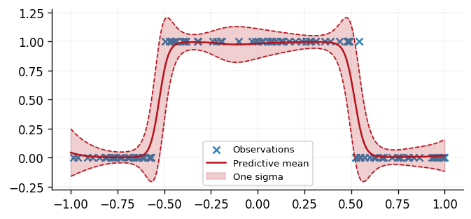
Here we projected the map estimates for the function values at the data points to get predictions over the whole domain,
However, as a point estimate, MAP estimation is severely limited for uncertainty quantification, providing only a single piece of information about the posterior.
Laplace approximation
The Laplace approximation improves uncertainty quantification by incorporating curvature induced by the marginal log-likelihood's Hessian to construct an approximate Gaussian distribution centered on the MAP estimate. Writing as the unormalised posterior for function values at the datapoints , we can expand the log of this about the posterior mode via a Taylor expansion. This gives:
Since is zero at the mode, this suggests the following approximation
that we identify as a Gaussian distribution, . Since the negative Hessian is positive definite, we can use the Cholesky decomposition to obtain the covariance matrix of the Laplace approximation at the datapoints below.
gram, cross_covariance = (kernel.gram, kernel.cross_covariance)
jitter = 1e-6

# Compute (latent) function value map estimates at training points:
Kxx = opt_posterior.prior.kernel.gram(x)
Kxx += identity_matrix(D.n) * jitter
Kxx = PSD(Kxx)
Lx = lower_cholesky(Kxx)
f_hat = Lx @ opt_posterior.latent[...]

# Negative Hessian,  H = -∇²p_tilde(y|f):
graphdef, params, *static_state = nnx.split(opt_posterior, Parameter, ...)


def loss(params, D):
    model = nnx.merge(graphdef, params, *static_state)
    return -gpx.objectives.log_posterior_density(model, D)


jacobian = jax.jacfwd(jax.jacrev(loss))(params, D)
H = jacobian["latent"]["latent"][...][:, 0, :, 0]
L = jnp.linalg.cholesky(H + identity_matrix(D.n) * jitter)

# H⁻¹ = H⁻¹ I = (LLᵀ)⁻¹ I = L⁻ᵀL⁻¹ I
L_inv = jsp.linalg.solve_triangular(L, identity_matrix(D.n), lower=True)
H_inv = jsp.linalg.solve_triangular(L.T, L_inv, lower=False)
LH = jnp.linalg.cholesky(H_inv)
laplace_approximation = npd.MultivariateNormal(f_hat.squeeze(), scale_tril=LH)
For novel inputs, we must project the above approximating distribution through the Gaussian conditional distribution ,
This is the same approximate distribution , but we have perturbed the covariance by a curvature term of . We take the latent distribution computed in the previous section and add this term to the covariance to construct .
def construct_laplace(test_inputs: Float[Array, "N D"]) -> npd.MultivariateNormal:
    map_latent_dist = opt_posterior.predict(xtest, train_data=D)

    Kxt = opt_posterior.prior.kernel.cross_covariance(x, test_inputs)
    Kxx = opt_posterior.prior.kernel.gram(x)
    Kxx += identity_matrix(D.n) * jitter
    Kxx = PSD(Kxx)

    # Kxx⁻¹ Kxt
    Kxx_inv_Kxt = solve(Kxx, Kxt)

    # Ktx Kxx⁻¹[ H⁻¹ ] Kxx⁻¹ Kxt
    laplace_cov_term = jnp.matmul(jnp.matmul(Kxx_inv_Kxt.T, H_inv), Kxx_inv_Kxt)

    mean = map_latent_dist.mean
    covariance = map_latent_dist.covariance_matrix + laplace_cov_term
    L = jnp.linalg.cholesky(covariance)
    return npd.MultivariateNormal(jnp.atleast_1d(mean.squeeze()), scale_tril=L)
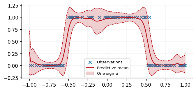
From this we can construct the predictive distribution at the test points.
laplace_latent_dist = construct_laplace(xtest)
predictive_dist = opt_posterior.likelihood(laplace_latent_dist)

predictive_mean = predictive_dist.mean
predictive_std = jnp.sqrt(predictive_dist.variance)

fig, ax = plt.subplots()
ax.scatter(x, y, label="Observations", color=cols[0])
ax.plot(xtest, predictive_mean, label="Predictive mean", color=cols[1])
ax.fill_between(
    xtest.squeeze(),
    predictive_mean - predictive_std,
    predictive_mean + predictive_std,
    alpha=0.2,
    color=cols[1],
    label="One sigma",
)
ax.plot(
    xtest,
    predictive_mean - predictive_std,
    color=cols[1],
    linestyle="--",
    linewidth=1,
)
ax.plot(
    xtest,
    predictive_mean + predictive_std,
    color=cols[1],
    linestyle="--",
    linewidth=1,
)
ax.legend()
<matplotlib.legend.Legend at 0x7efdc4c10750>
System configuration
Author: Thomas Pinder & Daniel Dodd

Last updated: Thu, 05 Mar 2026

Python implementation: CPython
Python version       : 3.11.14
IPython version      : 9.9.0

flax      : 0.12.2
gpjax     : 0.13.6
jax       : 0.9.0
jaxtyping : 0.3.6
matplotlib: 3.10.8
numpyro   : 0.19.0
optax     : 0.2.6

Watermark: 2.6.0