Deep Kernel Learning
In this notebook we demonstrate how GPJax can be used in conjunction with Equinox to build deep kernel Gaussian processes. Modelling data with discontinuities is a challenging task for regular Gaussian process models. However, as shown in , transforming the inputs to our Gaussian process model's kernel through a neural network can offer a solution to this.
import equinox as eqx
from examples.utils import use_mpl_style
from gpjax.kernels.computations import (
    AbstractKernelComputation,
    DenseKernelComputation,
)
import jax

# Enable Float64 for more stable matrix inversions.
from jax import config
import jax.numpy as jnp
import jax.random as jr
from jaxtyping import (
    Array,
    Float,
    install_import_hook,
)
import matplotlib as mpl
import matplotlib.pyplot as plt
import optax as ox
from scipy.signal import sawtooth

config.update("jax_enable_x64", True)


with install_import_hook("gpjax", "beartype.beartype"):
    import gpjax as gpx
    from gpjax.kernels.base import AbstractKernel


# set the default style for plotting
use_mpl_style()
cols = mpl.rcParams["axes.prop_cycle"].by_key()["color"]

key = jr.key(42)
Dataset
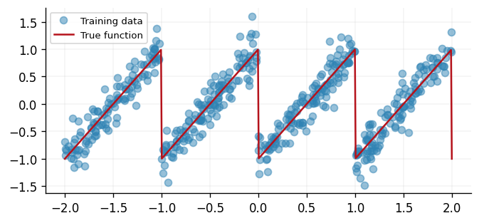
As previously mentioned, deep kernels are particularly useful when the data has discontinuities. To highlight this, we will use a sawtooth function as our data.
n = 500
noise = 0.2

key, subkey = jr.split(key)
x = jr.uniform(key=key, minval=-2.0, maxval=2.0, shape=(n,)).reshape(-1, 1)
f = lambda x: jnp.asarray(sawtooth(2 * jnp.pi * x))
signal = f(x)
y = signal + jr.normal(subkey, shape=signal.shape) * noise

D = gpx.Dataset(X=x, y=y)

xtest = jnp.linspace(-2.0, 2.0, 500).reshape(-1, 1)
ytest = f(xtest)

fig, ax = plt.subplots()
ax.plot(x, y, "o", label="Training data", alpha=0.5)
ax.plot(xtest, ytest, label="True function")
ax.legend(loc="best")
<matplotlib.legend.Legend at 0x7fbc59e6b6d0>
Deep kernels
Details
Instead of applying a kernel \(k(\cdot, \cdot')\) directly on some data, we seek to apply a feature map \(\phi(\cdot)\) that projects the data to learn more meaningful representations beforehand. In deep kernel learning, \(\phi\) is a neural network whose parameters are learned jointly with the GP model's hyperparameters. The corresponding kernel is then computed by \(k(\phi(\cdot), \phi(\cdot'))\). Here \(k(\cdot,\cdot')\) is referred to as the base kernel.
Implementation
Although deep kernels are not currently supported natively in GPJax, defining one is
straightforward as we now demonstrate. Inheriting from the base AbstractKernel
in GPJax, we create the DeepKernelFunction object that allows the
user to supply the neural network and base kernel of their choice. Kernel matrices
are then computed using the regular gram and cross_covariance functions.
class DeepKernelFunction(AbstractKernel):
    base_kernel: AbstractKernel
    network: eqx.Module

    def __init__(
        self,
        base_kernel: AbstractKernel = None,
        network: eqx.Module = None,
    ):
        self.base_kernel = base_kernel
        self.network = network
        super().__init__(compute_engine=DenseKernelComputation())

    def __call__(
        self, x: Float[Array, " D"], y: Float[Array, " D"]
    ) -> Float[Array, "1"]:
        xt = self.network(x)
        yt = self.network(y)
        return self.base_kernel(xt, yt)
Defining a network
With a deep kernel object created, we proceed to define a neural network. Here we consider a small multi-layer perceptron with two linear hidden layers and ReLU activation functions between the layers. The first hidden layer contains 64 units, whilst the second layer contains 32 units. Finally, we'll make the output of our network a three units wide. The corresponding kernel that we define will then be of ARD form to allow for different lengthscales in each dimension of the feature space. Users may wish to design more intricate network structures for more complex tasks, which functionality is supported well in Equinox.
feature_space_dim = 3


class Network(eqx.Module):
    layer1: eqx.nn.Linear
    output_layer: eqx.nn.Linear

    def __init__(
        self, key: jax.Array, *, input_dim: int, inner_dim: int, feature_space_dim: int
    ) -> None:
        key1, key2 = jr.split(key)
        self.layer1 = eqx.nn.Linear(input_dim, inner_dim, key=key1)
        self.output_layer = eqx.nn.Linear(inner_dim, feature_space_dim, key=key2)

    def __call__(self, x: jax.Array) -> jax.Array:
        x = self.layer1(x)
        x = jax.nn.relu(x)
        x = self.output_layer(x)
        return x


forward_linear = Network(
    jr.key(123), feature_space_dim=feature_space_dim, inner_dim=32, input_dim=1
)
Defining a model
Having characterised the feature extraction network, we move to define a Gaussian process parameterised by this deep kernel. We consider a third-order Matérn base kernel and assume a Gaussian likelihood.
base_kernel = gpx.kernels.Matern52(
    active_dims=list(range(feature_space_dim)),
    lengthscale=jnp.ones((feature_space_dim,)),
)
kernel = DeepKernelFunction(network=forward_linear, base_kernel=base_kernel)
meanf = gpx.mean_functions.Zero()
prior = gpx.gps.Prior(mean_function=meanf, kernel=kernel)
likelihood = gpx.likelihoods.Gaussian(num_datapoints=D.n)
posterior = prior * likelihood
Optimisation
We train our model via maximum likelihood estimation of the marginal log-likelihood. The parameters of our neural network are learned jointly with the model's hyperparameter set.
With the inclusion of a neural network, we take this opportunity to highlight the additional benefits gleaned from using Optax for optimisation. In particular, we showcase the ability to use a learning rate scheduler that decays the optimiser's learning rate throughout the inference. We decrease the learning rate according to a half-cosine curve over 700 iterations, providing us with large step sizes early in the optimisation procedure before approaching more conservative values, ensuring we do not step too far. We also consider a linear warmup, where the learning rate is increased from 0 to 1 over 50 steps to get a reasonable initial learning rate value.
schedule = ox.warmup_cosine_decay_schedule(
    init_value=0.0,
    peak_value=0.01,
    warmup_steps=75,
    decay_steps=700,
    end_value=0.0,
)

optimiser = ox.chain(
    ox.clip(1.0),
    ox.adamw(learning_rate=schedule),
)

opt_posterior, history = gpx.fit(
    model=posterior,
    objective=lambda p, d: -gpx.objectives.conjugate_mll(p, d),
    train_data=D,
    optim=optimiser,
    num_iters=800,
    key=key,
)
0%| | 0/800 [00:00<?, ?it/s]
Prediction
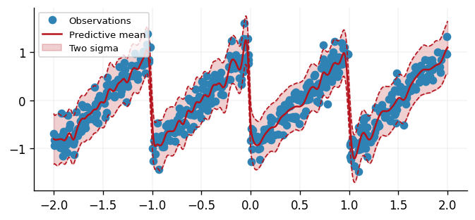
With a set of learned parameters, the only remaining task is to predict the output of the model. We can do this by simply applying the model to a test data set.
latent_dist = opt_posterior(xtest, train_data=D)
predictive_dist = opt_posterior.likelihood(latent_dist)

predictive_mean = predictive_dist.mean
predictive_std = jnp.sqrt(predictive_dist.variance)

fig, ax = plt.subplots()
ax.plot(x, y, "o", label="Observations", color=cols[0])
ax.plot(xtest, predictive_mean, label="Predictive mean", color=cols[1])
ax.fill_between(
    xtest.squeeze(),
    predictive_mean - 2 * predictive_std,
    predictive_mean + 2 * predictive_std,
    alpha=0.2,
    color=cols[1],
    label="Two sigma",
)
ax.plot(
    xtest,
    predictive_mean - 2 * predictive_std,
    color=cols[1],
    linestyle="--",
    linewidth=1,
)
ax.plot(
    xtest,
    predictive_mean + 2 * predictive_std,
    color=cols[1],
    linestyle="--",
    linewidth=1,
)
ax.legend()
<matplotlib.legend.Legend at 0x7fbc58afdb90>
System configuration
Author: Thomas Pinder

Last updated: Tue, 14 Jul 2026

Python implementation: CPython
Python version       : 3.11.15
IPython version      : 9.9.0

equinox   : 0.13.5
gpjax     : 0.17.0
jax       : 0.9.0
jaxtyping : 0.3.6
matplotlib: 3.10.8
optax     : 0.2.6
scipy     : 1.17.0

Watermark: 2.6.0
We currently have some availability for consulting on how Gaussian processes, Bayesian modelling, and GPJax can be integrated into your team's work. If this sounds relevant to your work, book an introductory call. These calls are for consulting inquiries only. For technical usage questions and free community support, please use GitHub Discussions and the documentation below.