Scalable Multi-Output GPs with OILMM

The multi-output notebook introduces the Intrinsic Coregionalisation Model (ICM) and the Linear Model of Coregionalisation (LCM), which capture cross-output correlations through coregionalisation matrices. Both approaches form the full joint covariance over all $n$ inputs and $p$ outputs. In the general case (LCM with $Q > 1$ components) this costs $\mathcal{O}((np)^3)$; even the single-component ICM, which enjoys Kronecker structure, still requires $\mathcal{O}(n^3 + p^3)$. When $p$ is large, both become prohibitively expensive from a computational and memory perspective.

The Orthogonal Instantaneous Linear Mixing Model (OILMM) of Bruinsma et al. (2020) resolves this bottleneck. It models the $p$ outputs as linear mixtures of $m \leq p$ latent Gaussian processes through a mixing matrix $\mathbf{H}$ whose columns are mutually orthogonal. This orthogonality causes the projected observation noise to be diagonal, which in turn allows inference to decompose into $m$ independent single-output GP problems. The overall cost drops to $\mathcal{O}(n^3 m)$ — linear in the number of latent processes and entirely independent of $p$.

This notebook derives the OILMM mathematics step by step, fits a model to three correlated North Atlantic wave-height outputs, optimises the model's parameters via the OILMM log marginal likelihood, and visualises its predictions.

from pathlib import Path

from examples.utils import use_mpl_style
from jax import config
import jax.numpy as jnp
import jax.random as jr
from jaxtyping import install_import_hook
import matplotlib as mpl
import matplotlib.pyplot as plt
import pandas as pd

config.update("jax_enable_x64", True)

with install_import_hook("gpjax", "beartype.beartype"):
    import gpjax as gpx

key = jr.key(123)
use_mpl_style()
cols = mpl.rcParams["axes.prop_cycle"].by_key()["color"]

The linear mixing model

A common formulation for multi-output GPs assumes that the $p$-dimensional output vector is generated by linearly mixing $m$ independent latent GPs:

\[ \mathbf{y}(t) = \mathbf{H}\,\mathbf{x}(t) + \boldsymbol{\varepsilon}(t), \]

where - $\mathbf{x}(t) = \bigl(x_1(t),\ldots,x_m(t)\bigr)^\top$ collects $m$ independent latent GPs, each with kernel $k_i$, - $\mathbf{H} \in \mathbb{R}^{p \times m}$ is the mixing matrix that maps from latent space to output space, and - $\boldsymbol{\varepsilon}(t) \sim \mathcal{N}\bigl(\mathbf{0},\,\sigma^2 \mathbf{I}_p\bigr)$ is i.i.d. observation noise.

Given $n$ input locations, we stack all observations into a vector $\bar{\mathbf{y}} \in \mathbb{R}^{np}$. Its joint covariance is

\[ \begin{aligned} \operatorname{cov}[\bar{\mathbf{y}}] = (\mathbf{H} \otimes \mathbf{I}_n)\, \operatorname{blkdiag}(\mathbf{K}_1,\ldots,\mathbf{K}_m)\, (\mathbf{H} \otimes \mathbf{I}_n)^\top + \sigma^2\,\mathbf{I}_{np}, \end{aligned} \]

where $\mathbf{K}_i$ is the $n \times n$ Gram matrix of the $i$-th latent kernel. Inverting this $np \times np$ matrix naively costs $\mathcal{O}(n^3 p^3)$, which is impractical when $p$ is even moderately large.

The OILMM parameterisation

OILMM constrains $\mathbf{H}$ to have orthogonal columns by writing

\[ \mathbf{H} = \mathbf{U}\,\mathbf{S}^{1/2}, \]

where $\mathbf{U} \in \mathbb{R}^{p \times m}$ has orthonormal columns ($\mathbf{U}^\top\mathbf{U} = \mathbf{I}_m$) and $\mathbf{S} = \operatorname{diag}(s_1,\ldots,s_m)$ with each $s_i > 0$ is a positive diagonal scaling matrix.

The corresponding projection matrix is the left pseudo-inverse of $\mathbf{H}$:

\[ \begin{aligned} \mathbf{T} &= \mathbf{S}^{-1/2}\,\mathbf{U}^\top, \\ \mathbf{T}\,\mathbf{H} &= \mathbf{S}^{-1/2}\, \underbrace{\mathbf{U}^\top\mathbf{U}}_{\mathbf{I}_m}\, \mathbf{S}^{1/2} = \mathbf{I}_m. \end{aligned} \]

Applying $\mathbf{T}$ to the observed outputs projects them into the latent space:

\[ \tilde{\mathbf{y}}(t) = \mathbf{T}\,\mathbf{y}(t) = \underbrace{\mathbf{T}\,\mathbf{H}}_{\mathbf{I}_m}\,\mathbf{x}(t) + \mathbf{T}\,\boldsymbol{\varepsilon}(t) = \mathbf{x}(t) + \tilde{\boldsymbol{\varepsilon}}(t). \]

Diagonal projected noise

The crux of OILMM is that the projected noise $\tilde{\boldsymbol{\varepsilon}} = \mathbf{T}\,\boldsymbol{\varepsilon}$ has a diagonal covariance:

\[ \operatorname{cov}[\tilde{\boldsymbol{\varepsilon}}] = \sigma^2\,\mathbf{T}\,\mathbf{T}^\top = \sigma^2\,\mathbf{S}^{-1/2}\, \underbrace{\mathbf{U}^\top\mathbf{U}}_{\mathbf{I}_m}\, \mathbf{S}^{-1/2} = \sigma^2\,\mathbf{S}^{-1}. \]

Because $\mathbf{S}$ is diagonal, the projected noise components are independent: the $i$-th latent observation has noise variance $\sigma^2/s_i$. This is the result that makes OILMM tractable.

GPJax additionally supports per-latent heterogeneous noise $\mathbf{D} = \operatorname{diag}(d_1,\ldots,d_m)$ with each $d_i \geq 0$. Including this term, the full projected noise covariance is

\[ \boldsymbol{\Sigma}_{\mathbf{T}} = \sigma^2\,\mathbf{S}^{-1} + \mathbf{D}, \]

which remains diagonal.

Independent latent inference

Because the projected noise is diagonal, each projected observation $\tilde{y}_i(t) = x_i(t) + \tilde{\varepsilon}_i(t)$ constitutes a standard single-output GP regression problem with known noise variance $\sigma^2/s_i + d_i$. We can therefore condition each latent GP independently using the standard conjugate formulae.

The cost of conditioning one GP on $n$ observations is $\mathcal{O}(n^3)$ (dominated by the Cholesky factorisation), so conditioning all $m$ latent GPs costs $\mathcal{O}(n^3 m)$. This is dramatically cheaper than the $\mathcal{O}(n^3 p^3)$ cost of the general linear mixing model.

Reconstructing predictions in output space

After conditioning, we obtain posterior means $\boldsymbol{\mu}_i$ and covariances $\boldsymbol{\Sigma}_i$ for each latent GP at $n_*$ test locations. The output-space predictive distribution is recovered by applying the mixing matrix:

\[ \begin{aligned} \boldsymbol{\mu}_{\mathbf{y}} &= \mathbf{H}\, \begin{pmatrix}\boldsymbol{\mu}_1 \\ \vdots \\ \boldsymbol{\mu}_m\end{pmatrix}, \\[6pt] \boldsymbol{\Sigma}_{\mathbf{y}} &= (\mathbf{H} \otimes \mathbf{I}_{n_*})\, \operatorname{blkdiag}(\boldsymbol{\Sigma}_1,\ldots, \boldsymbol{\Sigma}_m)\, (\mathbf{H} \otimes \mathbf{I}_{n_*})^\top. \end{aligned} \]

When only marginal variances are needed, the Kronecker product need not be formed explicitly. The marginal variance of output $j$ at test point $t$ is

\[ \operatorname{var}\bigl[f_j(t)\bigr] = \sum_{i=1}^{m} H_{ji}^2\,\operatorname{var}\bigl[x_i(t)\bigr], \]

which costs only $\mathcal{O}(n_* p\, m)$.

Atlantic wave data

We model hourly significant wave heights for December 2023 at a point in the North Atlantic west of Ireland (53.5°N, 11°W). The three outputs, measured in metres, are total wave height, swell, and wind sea. Swell is generated by distant storms, whereas wind sea responds to local winds; total wave height combines both drivers. Strictly, wave heights combine in energy — $H_{\text{total}} \approx \sqrt{H_{\text{swell}}^2 + H_{\text{wind}}^2}$ — so a linear mixture is an approximation, albeit one this data supports well. This gives the OILMM two meaningful latent processes to recover.

We subsample the ERA5 record, standardise time and each output for stable optimisation, and map predictions back to hours and metres for plotting. Note that the shared observation-noise variance $\sigma^2$ is homogeneous in standardised space; on the original scale this corresponds to a per-output noise floor of $\sigma^2 \operatorname{std}_j^2$.

Data: ERA5 wave reanalysis via Open-Meteo (CC-BY).

csv_candidates = [
    Path("examples/data/atlantic_wave_components.csv"),
    Path("data/atlantic_wave_components.csv"),
]
csv_path = next(path for path in csv_candidates if path.exists())
wave_frame = pd.read_csv(csv_path, parse_dates=["time"])

output_columns = ["wave_height", "swell_wave_height", "wind_wave_height"]
output_labels = ["Total wave height", "Swell", "Wind sea"]
num_outputs = len(output_columns)
num_latent = 2

subsample_stride = 3
wave_frame = wave_frame.iloc[::subsample_stride].reset_index(drop=True)
time_hours = (
    wave_frame["time"] - wave_frame["time"].iloc[0]
).dt.total_seconds().to_numpy() / 3600.0
wave_components_m = wave_frame[output_columns].to_numpy(dtype=float)

input_mean = time_hours.mean()
input_std = time_hours.std()
output_means = jnp.asarray(wave_components_m.mean(axis=0))
output_stds = jnp.asarray(wave_components_m.std(axis=0))

X_train = jnp.asarray(((time_hours - input_mean) / input_std).reshape(-1, 1))
y_train = (jnp.asarray(wave_components_m) - output_means) / output_stds
train_data = gpx.Dataset(X=X_train, y=y_train)


def plot_wave_output_panel(
    ax,
    output_index,
    train_hours,
    observations,
    labels,
    colors,
    test_hours=None,
    mean=None,
    func_std=None,
    obs_std=None,
):
    """Plot one wave component in physical units."""
    color = colors[output_index % len(colors)]
    ax.scatter(
        train_hours,
        observations[:, output_index],
        alpha=0.4,
        s=12,
        color=color,
        label="Training data",
    )
    if mean is not None:
        ax.plot(
            test_hours,
            mean[:, output_index],
            color=color,
            linewidth=2,
            label="Predictive mean",
        )
        if obs_std is not None:
            ax.fill_between(
                test_hours,
                mean[:, output_index] - 2 * obs_std[:, output_index],
                mean[:, output_index] + 2 * obs_std[:, output_index],
                alpha=0.14,
                color=color,
                label="Two sigma - observed output",
            )
        if func_std is not None:
            alpha = 0.26 if obs_std is not None else 0.2
            label = (
                "Two sigma - latent function"
                if obs_std is not None
                else "Two sigma"
            )
            ax.fill_between(
                test_hours,
                mean[:, output_index] - 2 * func_std[:, output_index],
                mean[:, output_index] + 2 * func_std[:, output_index],
                alpha=alpha,
                color=color,
                label=label,
            )
    ax.set_ylabel("wave height (m)")
    ax.set_title(labels[output_index])

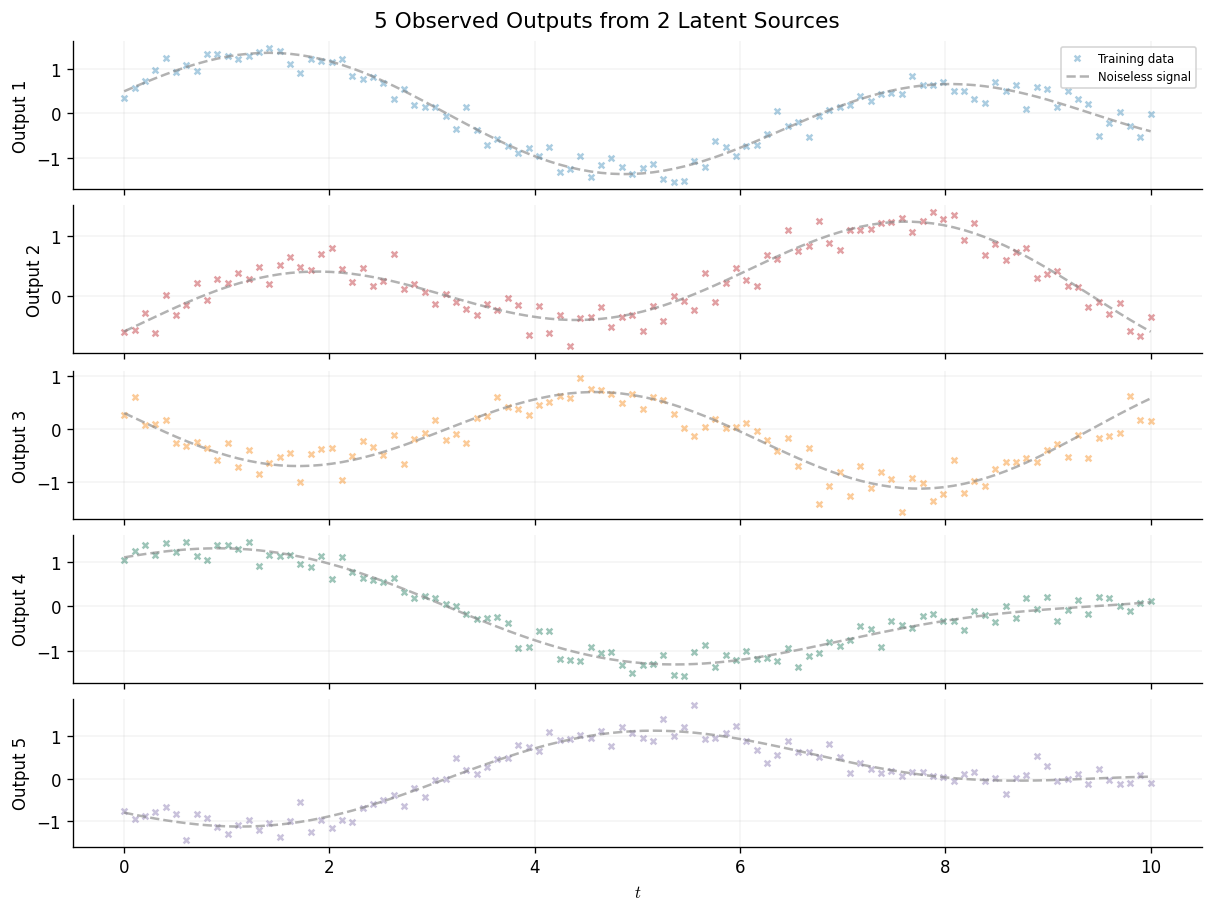
The total series rises with both component series, whilst swell and wind sea vary more independently. We fit two latent GPs so the mixing matrix can represent these distinct physical drivers.

fig, axes = plt.subplots(num_outputs, 1, figsize=(10, 6), sharex=True)

for output_index in range(num_outputs):
    plot_wave_output_panel(
        axes[output_index],
        output_index,
        time_hours,
        wave_components_m,
        output_labels,
        cols,
    )

axes[-1].set_xlabel("time (hours)")
axes[0].legend(loc="upper right", fontsize=7)
plt.suptitle("North Atlantic Wave Components", fontsize=13)

Text(0.5, 0.98, 'North Atlantic Wave Components')

png

Constructing the OILMM

GPJax provides create_oilmm_from_data, which initialises the mixing matrix using the empirical correlation structure of the outputs. Under the hood it first computes the empirical covariance matrix $$ \hat{\boldsymbol{\Sigma}} = \tfrac{1}{n-1}\,\mathbf{Y}_c^\top\mathbf{Y}_c, $$ where $\mathbf{Y}_c$ is the column-centred observation matrix. The next step extracts the top $m$ eigenvectors and eigenvalues of $\hat{\boldsymbol{\Sigma}}$. The function then sets $\mathbf{U}_{\text{latent}}$ to the eigenvectors. This ensures that after SVD orthogonalisation the columns of $\mathbf{U}$ align with the principal directions of output variation. Finally, $\mathbf{S}$ is set to the corresponding eigenvalues, giving the scaling an informative starting point. In this final step, the eigenvalues are floored at $10^{-6}$ for numerical stability.

This is analogous to initialising with PCA: the first $m$ principal components capture the most variance and provide a reasonable starting point for $\mathbf{H}$.

model = gpx.models.create_oilmm_from_data(
    dataset=train_data,
    num_latent_gps=num_latent,
    key=key,
    kernel=gpx.kernels.Matern52(),
)

Enforcing orthogonality via SVD

The OrthogonalMixingMatrix parameter stores an unconstrained matrix $\mathbf{U}_{\text{latent}} \in \mathbb{R}^{p \times m}$ and projects it onto the Stiefel manifold (the set of matrices with orthonormal columns) at each forward pass using SVD:

\[ \mathbf{U}_{\text{SVD}},\,\_,\,\mathbf{V}^\top = \operatorname{SVD}(\mathbf{U}_{\text{latent}}), \qquad \mathbf{U} = \mathbf{U}_{\text{SVD}}\,\mathbf{V}^\top. \]

This ensures $\mathbf{U}^\top\mathbf{U} = \mathbf{I}_m$ exactly, regardless of the optimiser's updates to the unconstrained representation.

U = model.mixing_matrix.U
UtU = U.T @ U
print(jnp.round(UtU, decimals=6))

[[ 1. -0.]
 [-0.  1.]]

Conditioning on observations

Before optimising any parameters, we condition with the PCA-initialised defaults to establish a baseline. Calling condition_on_observations executes the OILMM inference algorithm:

Project: compute $\tilde{\mathbf{Y}} = \mathbf{T}\,\mathbf{Y}^\top$ in $\mathcal{O}(nmp)$.
Condition: for each latent GP $i$, form a single-output dataset from $\tilde{\mathbf{y}}_i$ with noise variance $\sigma^2/s_i + d_i$, then condition using the standard conjugate formulae in $\mathcal{O}(n^3)$.
Return: an OILMMPosterior wrapping the $m$ independent posteriors.

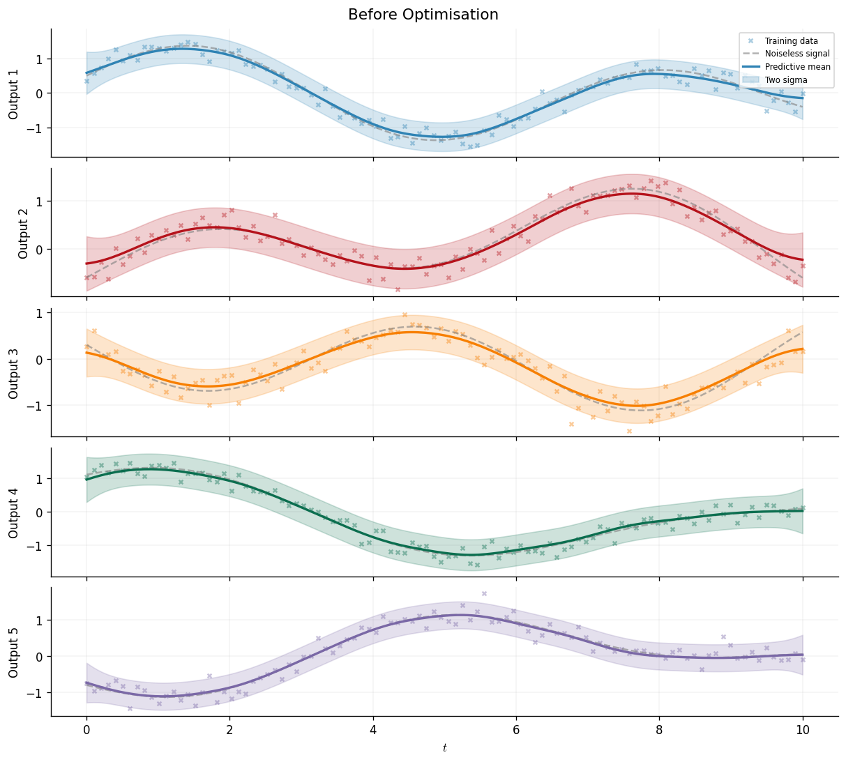
posterior = model.condition_on_observations(train_data)

Baseline predictions

We first inspect the model's output-space predictions using the default PCA-initialised parameters. This serves as a baseline against which we can later compare the optimised model.

N_test = 300
test_time_hours = jnp.linspace(
    float(time_hours.min()), float(time_hours.max()), N_test
)
X_test = ((test_time_hours - input_mean) / input_std).reshape(-1, 1)

pre_pred = posterior.predict(X_test, return_full_cov=False)
pre_opt_mean_standardised = pre_pred.mean.reshape(N_test, num_outputs)
pre_opt_std_standardised = jnp.sqrt(jnp.diag(pre_pred.covariance())).reshape(
    N_test, num_outputs
)
pre_obs_noise_var = (
    model.mixing_matrix.obs_noise_variance.unwrap()
    + model.mixing_matrix.H_squared @ model.mixing_matrix.latent_noise_variance.unwrap()
)
pre_obs_std_standardised = jnp.sqrt(
    pre_opt_std_standardised**2 + pre_obs_noise_var[None, :]
)

pre_opt_mean = pre_opt_mean_standardised * output_stds + output_means
pre_opt_std = pre_opt_std_standardised * output_stds
pre_obs_std = pre_obs_std_standardised * output_stds

fig, axes = plt.subplots(num_outputs, 1, figsize=(10, 6), sharex=True)

for output_index in range(num_outputs):
    plot_wave_output_panel(
        axes[output_index],
        output_index,
        time_hours,
        wave_components_m,
        output_labels,
        cols,
        test_time_hours,
        pre_opt_mean,
        func_std=pre_opt_std,
    )

axes[-1].set_xlabel("time (hours)")
axes[0].legend(loc="upper right", fontsize=7)
plt.suptitle("Before Optimisation", fontsize=13)

Text(0.5, 0.98, 'Before Optimisation')

png

OILMM log marginal likelihood

We optimise the model's parameters by maximising the OILMM log marginal likelihood. Proposition 9 of Bruinsma et al. (2020) gives the exact expression:

\[ \log p(\mathbf{Y}) = \underbrace{-\tfrac{n}{2}\log|\mathbf{S}|}_{\text{scaling penalty}} \;\underbrace{-\tfrac{n(p-m)}{2}\log(2\pi\sigma^2)}_{\text{residual noise}} \;\underbrace{-\tfrac{1}{2\sigma^2}\bigl\|(\mathbf{I}_p - \mathbf{U}\mathbf{U}^\top)\mathbf{Y}^\top\bigr\|_F^2}_{\text{projection residual}} \;+\;\sum_{i=1}^{m} \underbrace{\log\mathcal{N}\bigl(\tilde{\mathbf{y}}_i \mid \mathbf{0},\, \mathbf{K}_i + (\sigma^2/s_i + d_i)\mathbf{I}_n\bigr)}_{\text{latent GP marginal likelihood}}. \]

The first three terms are correction factors that account for the deterministic projection from output space to latent space:

Scaling penalty: penalises very large or small $s_i$ values, preventing the model from trivially inflating the likelihood by rescaling.
Residual noise: the log-probability of the $(p - m)$ directions orthogonal to $\mathbf{U}$, which are explained purely by observation noise.
Projection residual: the squared Frobenius norm of the data component that lies outside the column space of $\mathbf{U}$, divided by $\sigma^2$.

The final summation is simply the sum of $m$ standard single-output GP log marginal likelihoods, each evaluated on the projected data.

GPJax implements this in oilmm_mll(model, data), which takes the pre-conditioning OILMMModel (not a posterior) together with the training Dataset. We negate it for minimisation with fit_scipy.

initial_mll = gpx.models.oilmm_mll(model, train_data)

Optimisation

We maximise the OILMM log marginal likelihood using L-BFGS via fit_scipy. The optimiser tunes all array leaves: the kernel hyperparameters of each latent GP, the unconstrained mixing matrix $\mathbf{U}_{\text{latent}}$, the diagonal scaling $\mathbf{S}$, and the noise variances ($\sigma^2$ and $\mathbf{D}$).

opt_model, history = gpx.fit_scipy(
    model=model,
    objective=lambda m, d: -gpx.models.oilmm_mll(m, d),
    train_data=train_data,
    verbose=False,
)

opt_mll = gpx.models.oilmm_mll(opt_model, train_data)
print(f"Initial MLL: {initial_mll:.3f}")
print(f"Optimised MLL: {opt_mll:.3f}")

/home/runner/work/GPJax/GPJax/.venv/lib/python3.11/site-packages/scipy/optimize/_optimize.py:1474: RuntimeWarning: invalid value encountered in scalar multiply
  if (alpha_k*vecnorm(pk) <= xrtol*(xrtol + vecnorm(xk))):


Initial MLL: -926.295
Optimised MLL: -105.538

Post-optimisation predictions

We re-condition the optimised model on the training data, then predict at the same test locations.

opt_posterior = opt_model.condition_on_observations(train_data)
post_pred = opt_posterior.predict(X_test, return_full_cov=False)
post_opt_mean_standardised = post_pred.mean.reshape(N_test, num_outputs)
post_opt_std_standardised = jnp.sqrt(jnp.diag(post_pred.covariance())).reshape(
    N_test, num_outputs
)
post_obs_noise_var = (
    opt_model.mixing_matrix.obs_noise_variance.unwrap()
    + opt_model.mixing_matrix.H_squared
    @ opt_model.mixing_matrix.latent_noise_variance.unwrap()
)
post_obs_std_standardised = jnp.sqrt(
    post_opt_std_standardised**2 + post_obs_noise_var[None, :]
)

post_opt_mean = post_opt_mean_standardised * output_stds + output_means
post_opt_std = post_opt_std_standardised * output_stds
post_obs_std = post_obs_std_standardised * output_stds

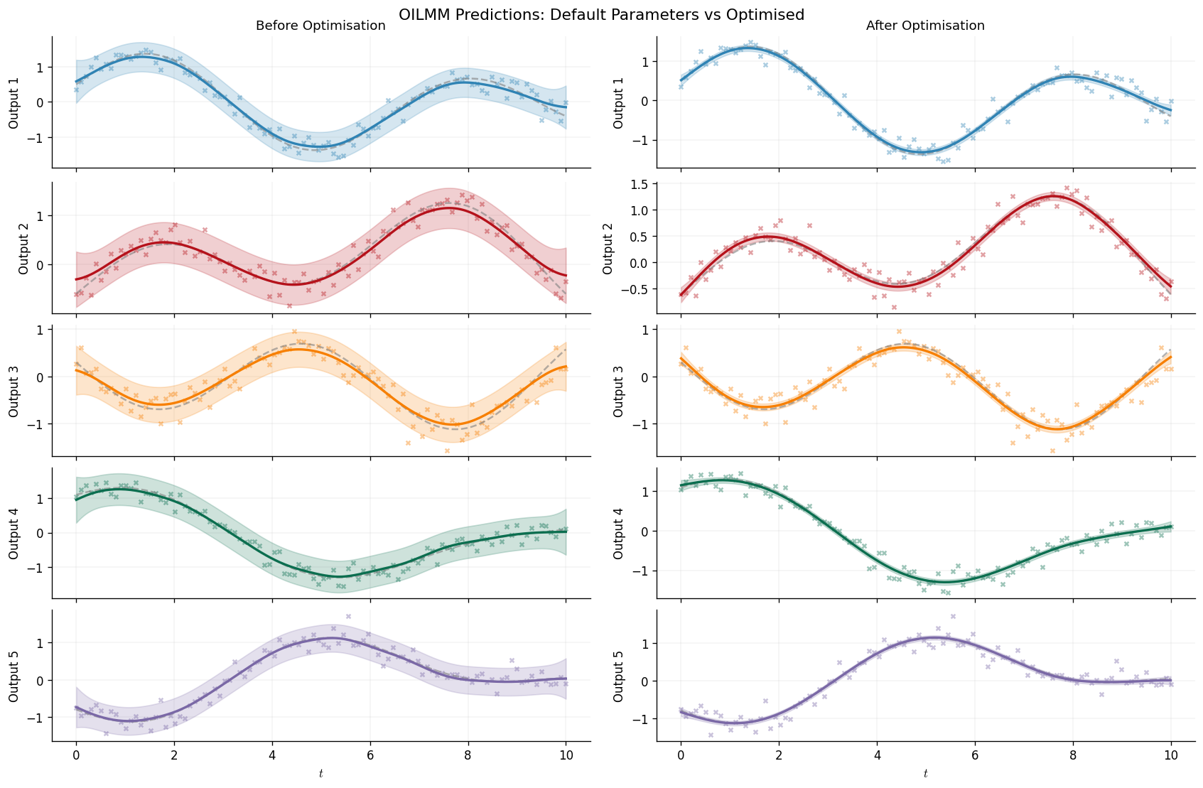
Before vs after comparison

We display the baseline (left) and optimised (right) predictions side by side for each wave component.

fig, axes = plt.subplots(num_outputs, 2, figsize=(14, 6), sharex=True)

for output_index in range(num_outputs):
    for column, (mean, std, title) in enumerate(
        [
            (pre_opt_mean, pre_opt_std, "Before Optimisation"),
            (post_opt_mean, post_opt_std, "After Optimisation"),
        ]
    ):
        plot_wave_output_panel(
            axes[output_index, column],
            output_index,
            time_hours,
            wave_components_m,
            output_labels,
            cols,
            test_time_hours,
            mean,
            func_std=std,
        )
        if output_index == 0:
            axes[output_index, column].set_title(
                f"{title}\n{output_labels[output_index]}", fontsize=11
            )
        if output_index == 0 and column == 1:
            axes[output_index, column].legend(loc="upper right", fontsize=7)

axes[-1, 0].set_xlabel("time (hours)")
axes[-1, 1].set_xlabel("time (hours)")
plt.suptitle("OILMM Wave Predictions: Default vs Optimised", fontsize=13, y=1.01)

Text(0.5, 1.01, 'OILMM Wave Predictions: Default vs Optimised')

png

Predictive uncertainty: latent function vs noisy observations

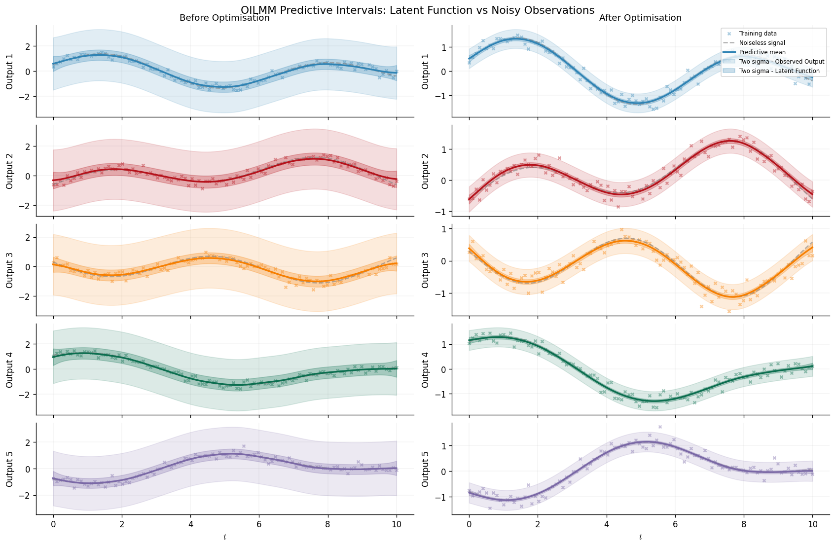
The previous figure shows uncertainty over the latent noise-free function $\mathbf{f}(t) = \mathbf{H}\mathbf{x}(t)$. To visualise uncertainty over observed outputs $\mathbf{y}(t)$, we add output-space noise:

\[ \operatorname{var}[y_j(t)] = \operatorname{var}[f_j(t)] + \sigma^2 + \sum_{i=1}^m H_{ji}^2 d_i. \]

The wider band below is the predictive standard deviation of noisy observations, whilst the narrower band is the latent function's standard deviation.

fig, axes = plt.subplots(num_outputs, 2, figsize=(14, 6), sharex=True)

for output_index in range(num_outputs):
    for column, (mean, function_std, observation_std, title) in enumerate(
        [
            (pre_opt_mean, pre_opt_std, pre_obs_std, "Before Optimisation"),
            (post_opt_mean, post_opt_std, post_obs_std, "After Optimisation"),
        ]
    ):
        plot_wave_output_panel(
            axes[output_index, column],
            output_index,
            time_hours,
            wave_components_m,
            output_labels,
            cols,
            test_time_hours,
            mean,
            func_std=function_std,
            obs_std=observation_std,
        )
        if output_index == 0:
            axes[output_index, column].set_title(
                f"{title}\n{output_labels[output_index]}", fontsize=11
            )
        if output_index == 0 and column == 1:
            axes[output_index, column].legend(loc="upper right", fontsize=7)

axes[-1, 0].set_xlabel("time (hours)")
axes[-1, 1].set_xlabel("time (hours)")
plt.suptitle(
    "OILMM Wave Intervals: Latent Function vs Noisy Observations",
    fontsize=13,
    y=1.01,
)

Text(0.5, 1.01, 'OILMM Wave Intervals: Latent Function vs Noisy Observations')

png

Latent space after optimisation

The decomposition into independent single-output problems is the heart of OILMM. We plot each latent GP's projected training data $\tilde{\mathbf{y}}_i$ alongside its posterior predictive distribution. These $m$ panels are completely independent — each latent GP knows nothing about the others.

Note that the latent functions are identified only up to a sign/scale ambiguity: flipping the sign of a column of $\mathbf{U}$ and the corresponding latent GP leaves the output-space predictions unchanged.

fig, axes = plt.subplots(1, num_latent, figsize=(5 * num_latent, 3), sharey=False)

for i in range(num_latent):
    ax = axes[i]
    lat_y = opt_posterior.latent_datasets[i].y.squeeze()
    ax.plot(
        time_hours, lat_y, "o", color=cols[i], alpha=0.4, ms=3, label="Projected data"
    )
    lat_pred = opt_posterior.latent_posteriors[i].predict(
        X_test, train_data=opt_posterior.latent_datasets[i]
    )
    lat_mean = lat_pred.mean
    lat_std = jnp.sqrt(jnp.diag(lat_pred.covariance()))

    ax.plot(
        test_time_hours, lat_mean, color=cols[i], linewidth=2, label="Posterior mean"
    )
    ax.fill_between(
        test_time_hours,
        lat_mean - 2 * lat_std,
        lat_mean + 2 * lat_std,
        color=cols[i],
        alpha=0.2,
        label="Two sigma",
    )
    ax.set_xlabel("time (hours)")
    ax.set_title(f"Latent GP {i + 1}")
    ax.legend(loc="best", fontsize=7)

png

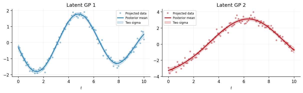
Each latent GP has learned a smooth function that explains the projected observations. The prediction intervals are narrow where data is dense and widen towards the boundaries. Crucially, these $m$ regression problems were solved independently, with total cost $\mathcal{O}(n^3 m)$.

Heterogeneous kernels

By default, passing a single kernel to OILMMModel deep-copies it $m$ times so that each latent GP has independent hyperparameters. If the latent processes operate at fundamentally different characteristic scales, you can go further and assign entirely different kernel families:

model = gpx.models.create_oilmm(
    num_outputs=3, num_latent_gps=2, key=key,
    kernel=[gpx.kernels.RBF(), gpx.kernels.Matern52()],
)

The first latent GP would then use an infinitely differentiable RBF kernel whilst the second uses the rougher Matern-5/2. This is analogous to the advantage of LCM over ICM in the multi-output setting, where different components can capture different spectral characteristics.

System configuration

%reload_ext watermark
%watermark -n -u -v -iv -w -a 'Thomas Pinder'

Author: Thomas Pinder

Last updated: Mon, 27 Jul 2026

Python implementation: CPython
Python version       : 3.11.15
IPython version      : 9.15.0

gpjax     : 0.18.0
jax       : 0.10.2
jaxtyping : 0.3.11
matplotlib: 3.11.1
pandas    : 3.0.0

Watermark: 2.6.0

We currently have some availability for consulting on how Gaussian processes, Bayesian modelling, and GPJax can be integrated into your team's work. If this sounds relevant to your work, book an introductory call. These calls are for consulting inquiries only. For technical usage questions and free community support, please use GitHub Discussions and the documentation below.